Adding bound/box constraints to any optimization method
There is a known trick for adding bound (a.k.a. box) constraints to optimization algorithms when the method does not natively support bound constraints, such as with the Levenberg-Marquardt algorithm. The trick is to simply add an internal scaling/transformation step in the objective function so that an unbound value is scaled into a bounded domain before actually being passed into the objective function. In this post we will examine the standard transformation used for this purpose, and examine the performance of some alternatives.
Let’s be formal for just a second. The goal is to transform an optimization problem of the form
\[\begin{gather*} & \min_{x} f(x) \end{gather*}\]to
\[\begin{gather*} & \min_{x} f(x)\\ & \textrm{s.t.} \quad l \leq x_{i} \leq u \end{gather*}\]which can be accomplished by applying a scaling function \(g\) to \(x\) prior to evaluation in \(f\), where \(g\) transforms \(x\) from an unbounded domain to some bound domain:
\[\begin{gather*} & \min_{x} f(g(x))\\ \end{gather*}\]The lmfit package uses the same
technique that the
MINUIT package uses. I’ve also seen
this strategy used elsewhere (i.e. in
this
modification of Matlab’s fminsearch method). The transformation involves
taking unbound values (used by the optimization algorithm) and transforming then
into the bound domain via:
Note that the approach is to take some function with limited range (\(sin(x)\) in this case, with a range of \((-1, 1)\)), shifting to a lower range of 0 (by adding 1 in this case) and scaling to an upper range of 1 (by dividing by 2 after the shift in this case), and then applying another scale factor of \(U- L\) where \(U\) is an arbitrary upper range and \(L\) is an arbitrary lower range, and ending with another shift of \(L\). Let’s look at the behavior of this transform over a dataset evenly spaced between -100 and 100 across 1000 steps, and transforming to a domain of \((0.1, 0.9)\):
import numpy as np
import matplotlib.pyplot as plt

def sin_scale(x, l, u, k=1./(2.*np.pi), x0=0.):
    return l + (u-l)*((np.sin(k*2.*np.pi*(x-x0))+1.)/2)

x_unbound = np.linspace(-100, 100, 1000)
x_bound = sin_scale(x_unbound, 0.1, 0.9)

plt.plot(x_unbound, x_bound)
plt.show(block=False)
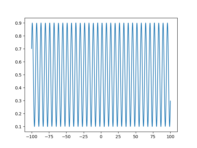
This sine transform is a highly redundant mapping to the bound domain. That is, going from -100 to 100 as in the example above, we would have explored the whole feasible domain of our parameter many times over. We could decrease the frequency of the sine wave to mitigate this a bit. Another approach would be to change the transform to a function that asymptotically approaches our bounds, i.e., a sigmoid function. With a sigmoid function, there will be no redundancy in the mapping to the bound domain, so increasing the unbound parameters used in the optimization routine will always increase the bound parameter seen by the objective function. A good candidate function for this transformation is the logistic function. We will use a particular form of the generalized logistic function so that we can set arbitrary asymptotic limits \(U\) and \(L\):
\[\begin{gather*} s(x_{unbound}) = L + (U - L) \frac{1} {1 + exp(-k(x_{unbound} - x_0))} \end{gather*}\]def logistic(x, l=0., u=1., k=1., x0=0.):
return l + (u-l)*(1/(1+np.exp(-k*(x-x0))))
x_bound = logistic(x_unbound, 0.1, 0.9)
plt.plot(x_unbound, x_bound)
plt.show(block=False)
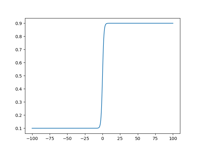
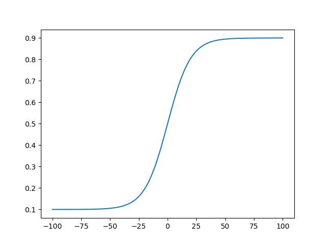
With the defaults this is just the standard logistic function, so the optimizer
will explore the majority of the bound domain when the unbound domain is around
0, but this can be spread out by modifying k.
x_bound = logistic(x_unbound, 0.1, 0.9, 0.1)

plt.plot(x_unbound, x_bound)
plt.show(block=False)
Another good candidate is
\[\begin{gather*} s(x_{unbound}) = \frac{x_{unbound}} {(1 + |x_{unbound}|^{k})^{1/k}} \end{gather*}\]which maps to \((-1, 1)\) and can be converted to map to an arbitrary domain in the same way as the previous functions:
\[\begin{gather*} s(x_{unbound}) = L + (U - L) \frac{1 + \frac{x_{unbound}} {(1 + |x_{unbound}|^{k})^{1/k}}} {2} \end{gather*}\]Note that, similar to the generalized logistic function, we can shift the
center point of this sigmoid (with an x0 parameter) and can change the growth
characteristic of the sigmoid with the k parameter.
def limit_scale(x, l=0., u=1., k=1., x0=0.):
    return l + (u-l)*(1 + ((x -x0) / (1+np.abs(x - x0)**k)**(1/k)))/2.
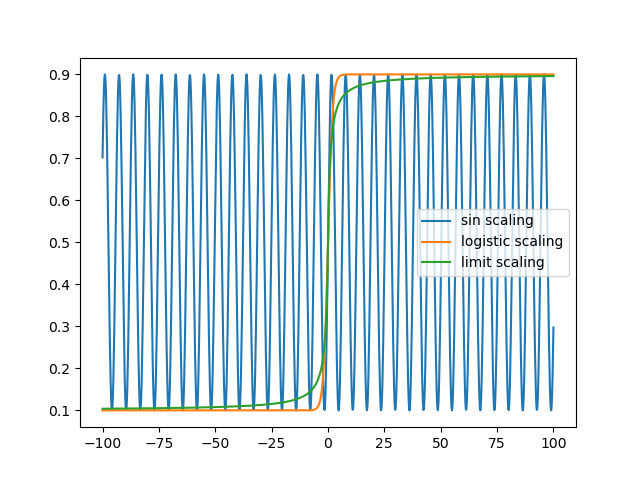
Let’s compare all of the scaling methods:
x_sin_scale = sin_scale(x_unbound, 0.1, 0.9)
x_logistic_scale = logistic(x_unbound, 0.1, 0.9)
x_limit_scale = limit_scale(x_unbound, 0.1, 0.9)

plt.plot(x_unbound, x_sin_scale, label = 'sin scaling')
plt.plot(x_unbound, x_logistic_scale, label = 'logistic scaling')
plt.plot(x_unbound, x_limit_scale, label = 'limit scaling')
plt.legend()
plt.show(block=False)
To compare the performance of the methods, I will generate noise free samples from an exponentially decaying sine wave with random parameters, and attempt to fit those parameters from the data.
u = 1.
l = 0.

def nonlinear_model(x, w):
    return w[0]*np.exp(-w[1]*x)*np.sin(2*np.pi*w[2]*x)

def obj_fun(ws, f=lambda a: a):
    return y - nonlinear_model(x, f(ws))

obj_fun_logistic = lambda ws: obj_fun(ws, lambda x: logistic(x, l, u))
obj_fun_sin = lambda ws: obj_fun(ws, lambda x: sin_scale(x, l, u))
obj_fun_limit = lambda ws: obj_fun(ws, lambda x: limit_scale(x, l, u))

logistic_res = []
sin_res = []
limit_res = []
unbound_res = []

true_pars = []

x = np.linspace(0,10*np.pi,1000)

for i in range(1000):
    np.random.seed(i)
    w = np.random.uniform(l, u, (3, ))
    true_pars.append(w)

    w_init = np.random.uniform(l, u, (3, ))

    y = nonlinear_model(x, w)

    res_unbound = opt.least_squares(obj_fun, w_init, method='lm')
    res_logistic = opt.least_squares(obj_fun_logistic, w_init, method='lm')
    res_sin = opt.least_squares(obj_fun_sin, w_init, method='lm')
    res_limit = opt.least_squares(obj_fun_limit, w_init, method='lm')

    logistic_res.append(res_logistic)
    sin_res.append(res_sin)
    limit_res.append(res_limit)
    unbound_res.append(res_unbound)
Here is an example of what we have fit:
ex_ind = 1
y = nonlinear_model(x, true_pars[ex_ind])
y_pred_logistic = nonlinear_model(x, logistic(logistic_res[ex_ind].x, l, u))
y_pred_sin = nonlinear_model(x, sin_scale(sin_res[ex_ind].x, l, u))
y_pred_limit = nonlinear_model(x, limit_scale(limit_res[ex_ind].x, l, u))
y_pred_unbound = nonlinear_model(x, unbound_res[ex_ind].x)

plt.figure(figsize=(10,10/4))
plt.subplot(1,4,1)
plt.plot(x, y, label = 'True Function')
plt.plot(x, y_pred_sin, label = 'Fit Function')
plt.legend(loc='upper right')
plt.title('Sine Scaling')

plt.subplot(1,4,2)
plt.plot(x, y)
plt.plot(x, y_pred_logistic)
plt.title('Logistic Scaling')

plt.subplot(1,4,3)
plt.plot(x, y)
plt.plot(x, y_pred_limit)
plt.title('Limit Scaling')

plt.subplot(1,4,4)
plt.plot(x, y)
plt.plot(x, y_pred_unbound)
plt.title('Unbound')
plt.tight_layout()
plt.show(block=False)
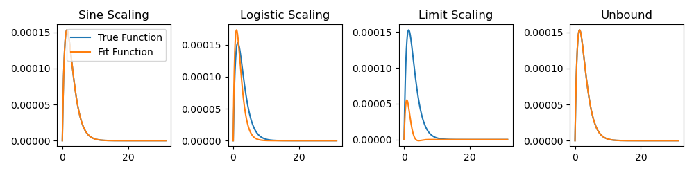
Note that, for clarity, I intentionally chose an example where some methods did
not converge to the correct solution. To get a better idea of the overall
performance of each method, we can save some key values, such as the number of
solutions with nonzero cost (meaning that we did not find the exact parameters),
stopping criteria (status parameters from the optimizer result object), etc.
sqrteps = np.sqrt(np.finfo('float64').eps)

logistic_nonzero_cost = [i.cost for i in logistic_res] > sqrteps
logistic_zero_cost = [i.cost for i in logistic_res] <= sqrteps
limit_nonzero_cost = [i.cost for i in limit_res] > sqrteps
limit_zero_cost = [i.cost for i in limit_res] <= sqrteps
sin_nonzero_cost = [i.cost for i in sin_res] > sqrteps
sin_zero_cost = [i.cost for i in sin_res] <= sqrteps
unbound_nonzero_cost = [i.cost for i in unbound_res] > sqrteps
unbound_zero_cost = [i.cost for i in unbound_res] <= sqrteps
In my simulation, there were 389 cases where the logistic method had nonzero cost, 87 cases where the limit scaling method had nonzero cost, 0 cases where the sin scaling had nonzero cost, and 1 case where the unbound method had nonzero cost. Focusing on the sigmoid functions, let’s look at the max fit parameters in cases with nonzero loss.
logistic_nonzero_res_vals = [logistic_res[i].x for i in [i for i, x in \
    enumerate(logistic_nonzero_cost) if x]]
logistic_zero_res_vals = [logistic_res[i].x for i in [i for i, x in \
    enumerate(logistic_zero_cost) if x]]
logistic_max_val_nonzero = [np.max(logistic(i, l, u)) for i in \
    logistic_nonzero_res_vals]
logistic_max_val_zero = [np.max(logistic(i, l, u)) for i in \
    logistic_zero_res_vals]

limit_nonzero_res_vals = [limit_res[i].x for i in [i for i, x in \
    enumerate(limit_nonzero_cost) if x]]
limit_zero_res_vals = [limit_res[i].x for i in [i for i, x in \
    enumerate(limit_zero_cost) if x]]
limit_max_val_nonzero = [np.max(limit_scale(i, l, u)) for i in \
    limit_nonzero_res_vals]
limit_max_val_zero = [np.max(limit_scale(i, l, u)) for i in \
    limit_zero_res_vals]

plt.boxplot([logistic_max_val_zero, logistic_max_val_nonzero, \
    limit_max_val_zero, limit_max_val_nonzero], labels = ['Logistic Zero',
    'Logistic Nonzero', 'Limit Zero', 'Limit Nonzero'])
plt.show(block=False)
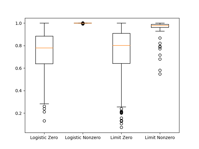
It seems like the failure of the sigmoid methods is related to approaching the upper limit in the scaling function. As that limit is approached, the derivative of the cost function with respect to the parameter approaches 0. The sine based scaling approach will not have this problem. One could envision some cases where the redundant mapping could affect the precision of the parameters estimates, since the whole feasible domain of the objective function is contained within such a small part of the scaling function. However, the standard method seems pretty reliable.