Second order methods for neural networks
High level packages for neural networks and optimization have greatly simplified the model development process. However, with these packages now becoming the “de facto” methods for approaching the task, the older methods are becoming something of a lost art. That is a bit of a problem because there are still many relevant cases where the classic approaches just seem to work better.
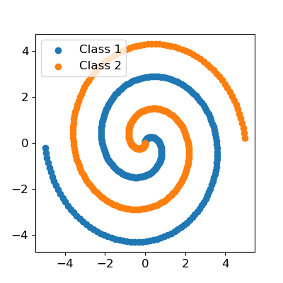
Consider the two spirals dataset, a pretty well known toy classification problem. In my experience, the modern packages actually have quite a bit of trouble with this dataset. Other people have also noted that this modeling task is not as straightforward as it seems, see here and here. One notable solution recommends a specific architecture with specific settings (using more specialized methods), and another recommends adding features (i.e. sine transformations of the inputs). So it can be done, but it is not straightforward. Not to mention that solutions like adding transformed features should not strictly be necessary, since ideally a neural network will learn this transform/mapping itself.
Somewhat analogously, I’ve seen numerous cases where a proven architecture and input set did not work as expected when translating a neural network model trained using classical optimization methods (i.e. Levenberg-Marquardt) to modern libraries (i.e. TensorFlow), which is usually done for the purpose of enabling GPU training. So it is sometimes the case that the same model architecture does not work “out of the box” with these newer packages. I believe this can largely be attributed to the fact that the new libraries are based solely on first-order, gradient descent type methods. “First-order” refers to the fact that the methods use only first derivative information, that is, calculation of the gradient of the model parameters (weights) with respect to the error function. However, you can obtain more information about the shape of the error function by considering the second derivative information (i.e. in the Hessian matrix), which can be used to obtain better optimization results. Without going into the details (perhaps that is for a discussion on another day), that is precisely what second order methods, such as the Levenberg-Marquardt algorithm, do. That’s not to say you can’t have issues using a second order method, but in my experience they tend to be a little more robust. Let’s explore that a bit. First, let’s load some dependencies for this analysis and generate a spiral dataset.
import matplotlib.pyplot as plt
import numpy as np
import tensorflow as tf
import scipy.optimize as opt

def spiral_data(nsamp):
    # Translated from
    # https://github.com/tensorflow/playground/blob/master/src/dataset.ts
    n = int(nsamp / 2)
    spiral_dat = np.zeros((nsamp, 4))
    cntr = 0
    # Generate the positive examples
    deltaT = 0
    for i in range(n):
        r = i / n * 5
        t = 1.75 * i / n * 2 * np.pi + deltaT
        x = r * np.sin(t)
        y = r * np.cos(t)
        spiral_dat[cntr,0] = x
        spiral_dat[cntr,1] = y
        spiral_dat[cntr,2] = 1
        cntr += 1
    # Generate the negative examples
    deltaT = np.pi
    for i in range(n):
        r = i / n * 5
        t = 1.75 * i / n * 2 * np.pi + deltaT
        x = r * np.sin(t)
        y = r * np.cos(t)
        spiral_dat[cntr,0] = x
        spiral_dat[cntr,1] = y
        spiral_dat[cntr,3] = 1
        cntr += 1
    return spiral_dat

spiral_dat = spiral_data(500)
fig = plt.figure()
fig.set_size_inches((5,5))
plt.scatter(spiral_dat[0:250,0], spiral_dat[0:250,1],
        label = "Class 1")
plt.scatter(spiral_dat[250:,0], spiral_dat[250:,1],
        label = "Class 2")
plt.xticks(fontsize = 12)
plt.yticks(fontsize = 12)
plt.legend(fontsize = 12)
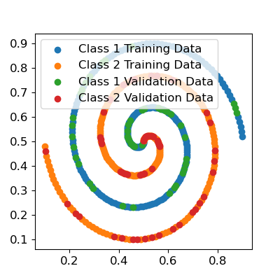
Let’s split this data into a training and validation set and scale it.
np.random.seed(0)
trn = np.random.choice(np.arange(0, spiral_dat.shape[0]),
         int(np.floor(spiral_dat.shape[0]*0.80)), replace = False)
val = np.setdiff1d(np.arange(0, spiral_dat.shape[0]), trn)

def linear_scale(data, scale_min, scale_max, data_min, data_max):
    # Allocate a matrix for the scaled data
    scaled_data = np.zeros((data.shape))
    for i in range(0, data.shape[1]):
        scaler = (scale_max[i] - scale_min[i]) / (data_max[i] - data_min[i])
        scaled_data[: ,i] = (scaler*(data[:, i] - data_min[i])) + scale_min[i]
    return scaled_data

spiral_inp_scaled = linear_scale(spiral_dat[:,0:2], np.array((0.1, 0.1)),
                                 np.array((0.9, 0.9)),
                                 np.max(spiral_dat[trn,0:2], axis = 0),
                                 np.min(spiral_dat[trn,0:2], axis = 0))
fig = plt.figure()
fig.set_size_inches((5,5))
plt.scatter(spiral_inp_scaled[np.intersect1d(trn, range(250)),0],
            spiral_inp_scaled[np.intersect1d(trn, range(250)),1],
            label = "Class 1 Training Data")
plt.scatter(spiral_inp_scaled[np.intersect1d(trn, range(250, 500)),0],
            spiral_inp_scaled[np.intersect1d(trn, range(250, 500)),1],
            label = "Class 2 Training Data")
plt.scatter(spiral_inp_scaled[np.intersect1d(val, range(250)),0],
            spiral_inp_scaled[np.intersect1d(val, range(250)),1],
            label = "Class 1 Validation Data")
plt.scatter(spiral_inp_scaled[np.intersect1d(val, range(250, 500)),0],
            spiral_inp_scaled[np.intersect1d(val, range(250, 500)),1],
            label = "Class 2 Validation Data")
plt.xticks(fontsize = 12)
plt.yticks(fontsize = 12)
plt.legend(fontsize = 12)
Now let’s fit a single hidden layer perceptron to the data using the Keras API. I’ll use 25 hidden nodes, and I’ll also initialize the model weights and biases myself so we can start from exactly the same point for the purposes of comparison. I will also set up a custom loss function to minimize the sum of squared errors, since the Levenberg-Marquardt algorithm exclusively minimizes the sum of squared errors. You can confirm you get similar final classification results with more conventional classification losses (i.e. categorical cross-entropy, or binary cross-entropy if you use just one of the two class labels and change the output activation function to a sigmoid).
# Initialize the model parameters
nin = 2
nhid = 25
nout = 2
npar_w1 = (nin+1)*nhid
np.random.seed(1)
ws_init = np.random.uniform(-0.1, 0.1, ((nin+1)*nhid) + ((nhid+1)*nout))
w_hid = np.reshape(ws_init[0:npar_w1], (nin+1, nhid), 'F')
w_out = np.reshape(ws_init[npar_w1:], (nhid+1, nout), 'F')
b_hid = w_hid[w_hid.shape[0]-1,:]
w_hid = w_hid[0:(w_hid.shape[0] - 1), :]
b_out = w_out[w_out.shape[0]-1,:]
w_out = w_out[0:(w_out.shape[0] - 1), :]

# Define the SSQ loss

def ssq(y_true, y_pred):
    return tf.reduce_sum(tf.square(y_true - y_pred))

# Fit the model
inp = tf.keras.layers.Input(shape = int(2))
inp_to_hid = tf.keras.layers.Dense(25, activation = 'sigmoid')
hid_to_out = tf.keras.layers.Dense(2, activation = 'softmax')
mdl = tf.keras.models.Model(inputs = inp, outputs
        = hid_to_out(inp_to_hid(inp)))
mdl.set_weights([w_hid, b_hid, w_out, b_out])
save_best = tf.keras.callbacks.EarlyStopping(monitor = 'val_loss', min_delta=0,
        patience=500, verbose=0, mode='min', baseline=None,
        restore_best_weights=True)
optmzr = tf.keras.optimizers.Adam(learning_rate = 1e-3)
mdl.compile(loss= ssq, optimizer=optmzr)
mdl.fit(x = spiral_inp_scaled[trn,0:2], y = spiral_dat[trn,2:],
        validation_data = (spiral_inp_scaled[val,0:2], spiral_dat[val,2:]),
        epochs = 10000, batch_size
        = len(trn), callbacks = save_best)

keras_preds = np.round(mdl.predict(spiral_inp_scaled[:,0:2]))

fig = plt.figure()
fig.set_size_inches((5,5))
plt.scatter(spiral_dat[keras_preds[:,0] == 1,0],
            spiral_dat[keras_preds[:,0] == 1,1],
        label = "Keras Predicted Class 1")
plt.scatter(spiral_dat[keras_preds[:,1] == 1,0],
            spiral_dat[keras_preds[:,1] == 1,1],
        label = "Keras Predicted Class 2")
plt.xticks(fontsize = 12)
plt.yticks(fontsize = 12)
plt.legend(fontsize = 12)
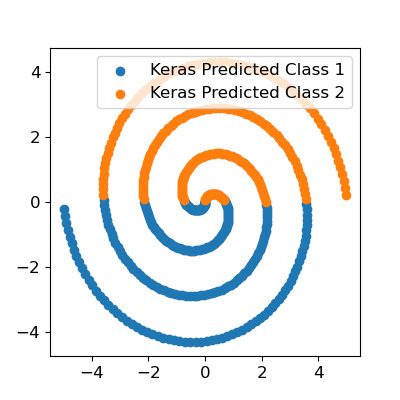
Clearly we’ve got some issues here - we did not fit the spiral at all. We do not even have any meaningful nonlinear separation in the input space. The optimizer just got stuck in a terrible local optimum.
Now let’s try to fit the same exact model with the Levenberg-Marquardt
algorithm. I will use the SciPy implementation from the
least_squares(method='lm') method. Obviously, this is not any sort of neural
network API, so we’ve got to set the implementation details up ourselves. For
instance, the method takes a vector of parameters, so we have to fold that
vector into the correct weight matrices in our custom perceptron function. To
keep things simple, I won’t write up an analytical gradient, I’ll just use the
default finite difference method in the Levenberg-Marquardt implementation.
First, set up our activation functions and custom perceptron functions:
def sig(x):
    return 1 / (1 + np.exp(-x))

def softmax(x):
    ex = np.exp(x)
    return ex / np.atleast_2d(np.sum(ex, axis = 1)).T

def mlp(x, ws, nhid, nout):
    # One hidden
    nin = x.shape[1]
    # Add 1 to account for bias nodes
    npar_w1 = (nin+1)*nhid
    npar_w2 = (nhid+1)*nout
    w_hid1 = np.reshape(ws[0:npar_w1], (nin+1, nhid), 'F')
    w_out = np.reshape(ws[npar_w1:], (nhid+1, nout), 'F')
    # Add constant to x for bias nodes
    x = np.hstack((x, np.ones((x.shape[0], 1))))
    hid1 = sig(np.matmul(x, w_hid1))
    # Again, need to add bias nodes to hidden layer
    hid1 = np.hstack((hid1, np.ones((hid1.shape[0], 1))))
    out = softmax(np.matmul(hid1, w_out))
    return out
Then, let’s write the optimization function (the function we will actually minimize). Again, the Levenberg-Marquardt algorithm is not a scalar minimization algorithm, it is strictly least squares. That is, it always minimizes the sum of squares, it is not compatible with any other loss function. Generally, with any call to a Levenberg-Marquardt implementation, you will return a vector of raw residuals (the difference between the true target values and current model predicted values), the sum of squares of which will be minimized.
def opt_fun(ws):
    y_trn = mlp(spiral_dat[trn,0:2], ws, nhid, nout)
    res = y_trn - spiral_dat[trn,2:4]
    trn_ssq = np.sum(res**2)
    res = res.flatten()
    # Print out the SSQs
    y_val = mlp(spiral_dat[val,0:2], ws, nhid, nout)
    val_ssq = np.sum((y_val - spiral_dat[val,2:])**2)
    print("Val SSQ : " + str(val_ssq))
    print("Trn SSQ : " + str(trn_ssq))
    return res
Finally, let’s fit the parameters. Note that you could write and pass in an analytic Jacobian function here (which you should in a real application - no one really fits neural networks with numerically calculated derivatives) but since this is just a simple test it’s not necessary.
sol = opt.least_squares(fun = opt_fun, x0 = ws_init, method = 'lm', max_nfev
        = 50000)
lm_preds = np.round(mlp(spiral_dat[:,0:2], sol.x, nhid, nout))

fig = plt.figure()
fig.set_size_inches((5,5))
plt.scatter(spiral_dat[lm_preds[:,0] == 1,0],
            spiral_dat[lm_preds[:,0] == 1,1],
        label = "LM Predicted Class 1")
plt.scatter(spiral_dat[lm_preds[:,1] == 1,0],
            spiral_dat[lm_preds[:,1] == 1,1],
        label = "LM Predicted Class 2")
plt.xticks(fontsize = 12)
plt.yticks(fontsize = 12)
plt.legend(fontsize = 12)
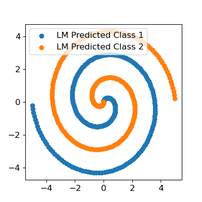
As you can see, we used exactly the same model architecture, initialized with the same weights, minimizing the same loss function, and obtained near-perfect classification, whereas TensorFlow failed. Now, it must be noted that there is a reason second order methods aren’t used exclusively. The first is that the methods are usually not amenable to minibatch training, just batch - thus, your data may not fit in memory. Another issue is model size. If the gradient vector contains \(n\) elements, the Hessian matrix, which contains the second derivative information, contains \(n^2\) elements. With a very large model, such as common deep learning models, this won’t fit in memory. However, with moderately sized data and moderately sized models, I believe second order methods should be the default over the various flavors of gradient descent.